
Содержание
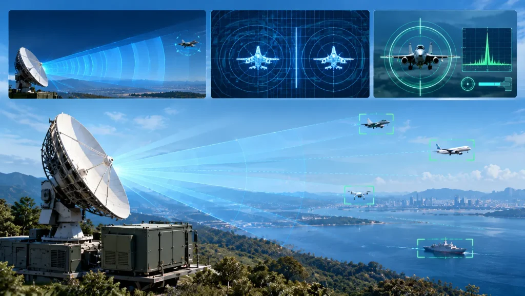
Radar range is the maximum distance at which a target can be detected, governed by the radar range equation and limited by the minimum detectable signal. Radar resolution is the ability to distinguish two closely spaced targets in range, angle, or velocity, determined by signal bandwidth and antenna aperture. Radar accuracy is how precisely a single target’s position (range, angle, velocity) can be measured, fundamentally limited by signal-to-noise ratio and system bandwidth. These three metrics are frequently conflated—but they answer fundamentally different questions, and confusing them leads to poor system design and worse procurement decisions.
1. Range: How Far Can the Radar See?
1.1 The Radar Range Equation
Maximum detection range is governed by the радар range equation, which balances transmitted power, antenna gain, target radar cross-section (RCS), and the minimum detectable signal. For a monostatic radar using the same antenna for transmit and receive, the received power at range R is:
Pr = Pt · G² · σ · λ² / [(4π)³ · R⁴]
Setting Pr equal to the minimum detectable signal Smin yields the maximum range:
Rmax = [Pt · G² · σ · λ² / ((4π)³ · Smin)]^(1/4)
The fourth-root dependence is the defining constraint of radar engineering. To double detection range, you must increase transmit power by a factor of 16—or increase antenna gain by 16, or reduce Smin by 16, or some combination. Every decibel of transmitter power, every decibel of receiver sensitivity, and every decibel of antenna gain translates directly into detection range—but at rapidly diminishing returns.
1.2 What Limits Range in Practice
The minimum detectable signal Smin is not a fixed number—it depends on receiver noise figure, system bandwidth, integration time, and the required signal-to-noise ratio for detection. A lower noise figure directly lowers Smin, extending range without increasing transmit power. This is why the first-stage low-noise amplifier in a radar receiver is one of the most consequential components in the entire system: its noise figure establishes the noise floor against which every target return must compete.
Losses also matter. The complete radar equation includes system losses L (feed losses, atmospheric attenuation, processing losses), and the SNR at the receiver is:
SNR = Pt · G² · λ² · σ / [(4π)³ · R⁴ · k · T₀ · B · Fn · L]
where k is Boltzmann’s constant, T₀ is reference temperature, B is receiver bandwidth, and Fn is the receiver noise figure. Every term in the denominator degrades range. The engineering challenge is minimizing each one without sacrificing the others.
2. Resolution: How Well Can the Radar Separate Targets?
2.1 Range Resolution: Bandwidth Is Everything
Range resolution is the minimum separation in range at which two targets can be distinguished. It is determined by the bandwidth of the transmitted waveform:
where c is the speed of light and B is the signal bandwidth. A 10 MHz bandwidth gives roughly 15 meters of range resolution; a 500 MHz bandwidth gives roughly 0.3 meters.
This relationship creates a fundamental tension. A short pulse provides high bandwidth and fine range resolution, but carries little energy—and therefore short detection range. A long pulse carries more energy for long-range detection, but has narrow bandwidth and poor range resolution.
Pulse compression resolves this tension. By modulating a long pulse with linear frequency modulation (or phase coding), the transmitted waveform achieves the energy of a long pulse while the matched filter on receive compresses it to a duration equivalent to a short pulse. A 100-microsecond chirp with 10 MHz bandwidth compresses to an effective pulse width of 0.1 microseconds—delivering both long-range energy and fine range resolution. The compression ratio equals the time-bandwidth product.
The implication for RF front-end design is significant: pulse compression demands high linearity and low phase noise. Non-linearities corrupt the modulated waveform, raising sidelobes that can mask weak targets; phase noise degrades the coherence of the compression process.
2.2 Angular Resolution: Aperture Governs
Angular resolution—the ability to separate two targets at the same range but different angles—is determined by the antenna beamwidth, which in turn depends on the physical aperture (or, for arrays, the effective aperture):
where λ is the wavelength and D is the aperture dimension. A larger aperture produces a narrower beam and finer angular resolution. For a uniform linear array with M elements spaced d apart, the effective aperture is D = M·d, and the angular resolution improves as the aperture grows.
This is one reason why phased-array radars can achieve angular resolution far beyond what a single mechanically scanned antenna of comparable physical size could deliver: the effective aperture can be synthesized through coherent processing across many elements. Synthetic aperture radar (SAR) takes this principle to its logical extreme, synthesizing an aperture many times larger than the physical antenna by coherently combining returns collected along a flight path.
The trade-off is direct: finer angular resolution requires larger apertures, more elements, and more T/R channels—driving up cost, power consumption, and integration complexity. For a given aperture, higher frequency (shorter wavelength) also improves angular resolution, but at the cost of greater atmospheric attenuation.
3. Accuracy: How Precisely Can the Radar Measure?
3.1 Accuracy Is Not Resolution
The distinction between accuracy and resolution is fundamental and frequently misunderstood.
Резолюция is the ability to distinguish two targets that are close together—the minimum separation at which they appear as separate detections rather than a single merged return.
Точность is the absolute correctness with which a single target’s position is measured—the difference between the measured value and the true value.
Two targets can be well resolved but poorly measured: the radar separates them clearly, but both range estimates are off by several meters. Conversely, a single target can be accurately measured but not resolved from a nearby second target: the centroid of the combined return is precisely estimated, but it does not correspond to either target’s true position.
A critical practical implication: resolution is fundamentally limited by hardware (bandwidth, aperture, wavelength), while accuracy can often be improved through signal processing. Zero-padding the frequency spectrum, for example, can improve interpolation accuracy without changing the underlying resolution. But no amount of processing can overcome the physical resolution limit imposed by bandwidth and aperture.
3.2 What Governs Range Accuracy
The theoretical lower bound on range measurement error is given by the Cramér-Rao lower bound (CRLB). For a radar with bandwidth B and signal-to-noise ratio SNR, the range accuracy σR satisfies:
σR ≥ c / (2 · √(SNR · B²)) = c / (2 · B · √SNR)
This expression reveals two levers for improving range accuracy:
Bandwidth. Accuracy improves inversely with bandwidth—the same bandwidth that determines resolution also determines the achievable accuracy ceiling. This is why wideband radar systems are valued not only for resolution but for precision measurement.
Signal-to-noise ratio. Accuracy improves with the square root of SNR. Every 6 dB improvement in SNR roughly doubles range accuracy. SNR is determined by transmit power, antenna gain, receiver noise figure, integration time, and target RCS—the same factors that govern detection range.
In practice, range accuracy is also limited by timing jitter, clock stability, and calibration errors. A system with excellent SNR but poor timing coherence will not achieve its theoretical accuracy bound.
3.3 What Governs Angular Accuracy
Angular accuracy follows a different scaling law. For a monopulse or beam-splitting angle estimator, the angular error is proportional to the beamwidth divided by the square root of SNR:
σθ ∝ θB / √SNR
With 20 dB SNR, the RMS angle error is roughly one-twentieth of a beamwidth; at 28 dB, roughly one-fiftieth. Achieving 0.1 milliradian accuracy may require SNR of 40 dB or higher.
This means angular accuracy is improved by the same levers that improve angular resolution—narrower beams, larger apertures—plus higher SNR. The difference is that resolution depends on the beamwidth itself, while accuracy depends on how precisely the angle of arrival can be estimated within that beamwidth—a parameter that can be improved through monopulse processing, array signal processing, and calibration.
4. The Engineering Trade-Off Triangle
Range, resolution, and accuracy are not independent—they trade against one another and against system resources:
| Metric | Primary Determinants | Improvement Lever | Penalty |
|---|---|---|---|
| Maximum Range | Pt, G, σ, Smin (noise figure) | More power, lower NF, larger antenna | Cost, size, power, thermal load |
| Разрешение по дальности | Bandwidth B | Wider bandwidth, pulse compression | Processing load, spectrum allocation, front-end linearity |
| Angular Resolution | Aperture D / wavelength λ | Larger aperture, more elements, higher frequency | Cost, integration density, T/R channel count |
| Range Accuracy | B, SNR | Wider bandwidth, higher SNR, better timing | Same as resolution + power |
| Angular Accuracy | Beamwidth, SNR | Narrower beam, higher SNR, monopulse processing | Aperture size, channel count, calibration complexity |
A radar optimized for maximum range—high power, large antenna, narrow bandwidth—will generally have poor range resolution. A radar optimized for fine resolution—wide bandwidth, pulse compression—demands high linearity and low phase noise throughout the signal chain. A radar optimized for angular accuracy—large aperture, many channels—demands consistent amplitude and phase across every T/R path.
There is no free parameter. Every improvement in one dimension imposes a cost elsewhere—in power, size, cost, thermal complexity, or signal processing burden. The engineer’s task is to find the operating point that matches the mission.
5. Why the RF Front-End Determines All Three
The performance limits of range, resolution, and accuracy are established at the RF front-end before any signal processing occurs.
Дальность обнаружения is set by the noise floor, and the noise floor is dominated by the first-stage low-noise amplifier. A receiver with a noise figure of 0.35 dB presents a fundamentally lower Smin than one with 2 dB—translating directly into extended detection range without any increase in transmit power.
Range resolution and accuracy depend on waveform bandwidth and linearity. Pulse compression demands that the transmitter reproduce the modulated waveform faithfully and that the receiver preserve its spectral shape. Non-linearities raise sidelobes and corrupt the compression process; phase noise degrades coherence.
Angular resolution and accuracy depend on the aperture and on the consistency of every channel behind it. In a phased array, each element’s T/R module must deliver matched amplitude and phase response; any deviation degrades beamforming quality and angular precision.
Transmit power sets the energy available for detection, and the efficiency with which that power is generated determines the thermal burden the system must bear. GaN power devices offer higher power density and thermal stability than legacy technologies, enabling higher transmit power within constrained platform volumes—but only if the thermal path is engineered to match.
6. STARDL’s RF Front-End Portfolio for Range, Resolution, and Accuracy
STARDL’s RF and microwave IC portfolio addresses the three performance pillars at the component level:
Силовые устройства на основе GaN cover 0.5 GHz to 8.0 GHz with output power up to 100W, featuring pre-matched internal impedance networks that maintain stable linearity under pulsed and continuous-wave operation. Higher transmit power directly extends maximum range under the fourth-root law—and GaN’s thermal stability supports sustained operation without derating that would erode that advantage.
Low-Noise Amplifiers (GaAs process) achieve noise figures as low as 0.35 dB, lowering Smin and extending detection range without additional transmit power. In a pulse-compression radar, the LNA must also preserve linearity across the wide instantaneous bandwidth—a requirement STARDL’s LNA designs address through careful input matching and bias optimization.
RF and Microwave ICs span DC to 50 GHz, including mixers, multipliers, phase shifters, and attenuators, providing the signal-chain functions that preserve waveform fidelity and phase coherence. Phase noise and linearity at these stages directly determine whether the theoretical resolution and accuracy limits are approached in practice.
Packaged ICs and T/R Modules support high-density integration with consistent channel-to-channel performance. For phased-array systems, where angular resolution and accuracy depend on aperture coherence, STARDL’s T/R module expertise addresses the core challenge of maintaining amplitude and phase consistency across many channels in a constrained volume.
Голый кристалл options eliminate package parasitics for designs where every fraction of a decibel of loss and every picosecond of timing skew matters—particularly at millimeter-wave frequencies where range accuracy is most sensitive to front-end imperfections.
Реальность инженерного дела
Range, resolution, and accuracy are the three axes on which radar performance is measured. They answer different questions: How far can I see? How finely can I separate? How precisely can I measure? They are governed by different physical mechanisms—the fourth-root range law, the bandwidth-resolution relationship, the aperture-angle relationship, and the SNR-accuracy scaling.
But they share a common foundation: the RF front-end. Transmit power and efficiency set the energy budget; noise figure sets the detection floor; linearity and phase noise preserve waveform fidelity; channel consistency preserves aperture coherence. No signal processing algorithm can recover performance that the front-end has already discarded.
STARDL’s portfolio—GaN power devices, GaAs LNAs, RF microwave ICs, packaged devices, and T/R modules—addresses these front-end determinants across the frequency range from DC to 50 GHz, providing radar designers with the building blocks to push range, resolution, and accuracy toward their physical limits.