
Índice
First: What physical mechanism is used to amplify or switch signals? (Process & Device Physics)
Second: How are these physical mechanisms organized into a usable circuit? (Topology & Architecture)
Third: Under the constraints of high frequency, high temperature, and high power, how do we ensure this circuit works reliably and repeatably? (Engineering & Manufacturing)
This article follows these three layers of logic.
1. Layer One: Device Physics – How Does a Transistor Actually Amplify?
The most critical active device in an RF chip is the field‑effect transistor (FET). Whether it is called HEMT, pHEMT, or MOSFET, the fundamental mechanism of signal amplification remains the same: controlling the channel current through the gate voltage.
However, the efficiency of this “control” varies dramatically across different process technologies.
1.1 GaAs HEMT – Electrons Run Fast
The core of a HEMT (High Electron Mobility Transistor) is the heterojunction – two semiconductor materials with different bandgaps grown together, forming a two‑dimensional electron gas (2DEG) at the interface. This electron gas has extremely high mobility because the electrons do not collide with impurity atoms at the interface.
The electron mobility of GaAs HEMT can exceed 8000 cm²/(V·s) . This means that for the same change in gate voltage, the channel current changes more – higher transconductance and better frequency performance.
Another advantage of GaAs HEMT is its noise performance. Because electron‑phonon scattering in the channel is weaker, both channel thermal noise and flicker noise are lower than in silicon‑based devices. This is why almost all high‑end receive‑chain LNAs choose GaAs pHEMT – its physical structure is inherently “low‑noise.”
1.2 GaN HEMT – Withstands High Voltage
The bandgap of GaN é 3.4 eV, compared to 1.4 eV for GaAs. The direct consequence is that GaN’s breakdown field strength is an order of magnitude higher than that of GaAs.
What does higher breakdown field mean? For the same transistor size, GaN can tolerate much higher drain voltage – thus delivering much higher output power. Power density is several times that of GaAs. A 2022 comparative study explicitly states that GaN HEMT shows higher power and frequency capability in terms of the modified Johnson figure‑of‑merit (based on cut‑off frequency).
Another advantage of GaN is thermal stability. Over a temperature range of –40°C to +150°C, the small‑signal model parameters of GaN HEMT vary far less than those of GaAs devices. This means that in high‑power, high‑temperature environments like radar transmitters, GaN reliability is far superior to GaAs.
The trade‑off between GaAs and GaN is fundamentally a trade‑off of physical laws: GaAs gives low noise and high linearity; GaN gives high power density and high temperature tolerance. There is no “better” – only “more suitable.”
2. Layer Two: Circuit Architecture – From Transistor to Functional Block
A transistor alone is just an amplifying element – it must be organized into specific circuit topologies to perform functions like amplification, mixing, and switching.
2.1 Architectural Logic of Low‑Noise Amplifiers (LNA)
The core design challenge of an LNA is the conflict between noise matching and power matching.
For a given transistor, the source impedance that yields minimum noise figure and the one that yields maximum gain typically do not coincide. The designer must plot two circles on the Smith chart – a constant noise‑figure circle and a constant gain circle – and find a compromise.
In circuit implementation:
- Source inductive degeneration is the classic input matching structure for LNAs. By placing a small inductor in series with the source, the real part of the input impedance can be pulled to 50Ω without increasing noise.
- Cascode topology is a common choice to improve bandwidth and isolation. The common‑gate stage eliminates the Miller effect, flattening high‑frequency gain.
2.2 Architectural Logic of Power Amplifiers (PA)
The core design challenge of a PA is the eternal conflict between efficiency and linearity.
The physical root of this conflict lies in the transistor’s operating region:
| Class | Conduction Angle | Theoretical Efficiency | Linearity |
|---|---|---|---|
| A | 360° | ≤50% | Best |
| AB | 180°–360° | 50%–78.5% | Good |
| B | 180° | 78.5% | Crossover distortion |
| C | <180° | >78.5% | Poor |
Class‑A amplifiers offer the best linearity, but the theoretical maximum efficiency is only 50% – the other 50% of DC power becomes heat. Class‑C amplifiers can achieve very high efficiency, but the output signal is severely distorted.
Engineering approaches to mitigate this trade‑off include:
Doherty architecture: Uses two transistors – the main amplifier operates alone at low power, and the auxiliary amplifier kicks in at high power. This architecture maintains relatively high efficiency even in power back‑off regions, making it the dominant choice for base‑station PAs.
Power back‑off: Operating the PA far below its saturated output power to exchange efficiency for linearity. However, the penalty is a sharp drop in efficiency.
Digital pre‑distortion (DPD): Before the signal enters the PA, a distortion inverse to the PA’s nonlinear characteristics is pre‑applied, and the two cancel out to produce a linear output.
2.3 Architectural Logic of Mixers and Switches
The core of a mixer is nonlinearity – using the nonlinear characteristics of transistors to multiply two signals of different frequencies, producing sum and difference frequencies.
- Passive mixers use diodes or switch‑type transistors. They offer good linearity and low noise, but require high local‑oscillator drive power.
- Active mixers use transistors to provide gain. They offer higher integration but slightly worse noise and linearity.
The core of an RF switch is the trade‑off between isolation and insertion loss. From SPDT to SP6T, insertion loss increases with the number of ports. STARDL’s high‑isolation digital RF switches (up to SP6T) maintain low insertion loss and high isolation from DC to 40 GHz. The design goal is to simultaneously minimise insertion loss and maximise isolation across a wide frequency range.
3. Layer Three: Engineering & Manufacturing – Why Datasheet Parameters Do Not Match Board Performance
This is the most common frustration for RF engineers: the S‑parameters on the datasheet are measured on a wafer‑level probe station – probes directly contacting the chip’s pads. But on your PCB, the chip goes through packaging, wire bonding, and traces – each step introduces additional parasitic parameters.
3.1 Parasitic Effects – The “Invisible Killer” of RF Circuits
At GHz frequencies, physical trace dimensions are already comparable to the signal wavelength. A 1‑mm bond wire has an inductance of approximately 1 nH at 10 GHz, presenting an inductive reactance of about 63 Ω – close to the system’s characteristic impedance. This means the bond wire itself alters the circuit’s matching condition.
What makes RFIC design special is that parasitic effects are first‑order, not second‑order influences on performance. This is why RFIC design requires iterative electromagnetic simulation, parasitic extraction, and package modelling throughout the entire design process.
3.2 Temperature Drift – The Underestimated Performance Killer
Datasheet typical values are measured at room temperature (25°C) . But your system may need to operate from –40°C to +85°C or even wider.
A 2016 study compared the small‑signal parameter variations of GaAs and GaN HEMTs over the –40°C to 150°C range. The conclusion: the temperature coefficients of the two device types are completely different. The intrinsic capacitances of GaAs change significantly with temperature, while those of GaN change much less.
This means: GaAs devices require larger performance margins across temperature, while GaN’s stability at high temperatures is a physical advantage.
3.3 Grounding and Decoupling – The Most Overlooked “System Problem”
O return path of an RF signal must closely follow the signal path. If the ground impedance is too high or the loop path is too long, a large loop is formed, introducing radiation and coupling.
Decoupling capacitor selection is not simply “the bigger, the better.” RF chips – especially PAs in pulsed mode – draw dynamic current. Different frequencies of noise require different capacitance values to filter, typically requiring a combination across three orders of magnitude (pF, nF, µF).
4. Back to STARDL’s Product Logic
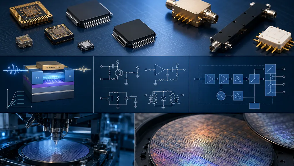
STARDL’s RF and microwave IC portfolio – ranging from bare die to packaged devices to GaN power devices – covers the DC to 50 GHz frequency spectrum. The three product categories address distinct engineering scenarios:
Matriz nua – Designed for design teams that pursue ultimate performance and have micro‑assembly capabilities. Removing the package eliminates parasitics, but users must handle bonding and assembly themselves.
Packaged ICs – Designed for high‑efficiency, high‑reliability volume production. Ceramic packaging suits military and aerospace applications; plastic packaging suits high‑volume commercial production.
GaN Power Devices – Designed for radar transmitters and electronic warfare systems that require “high‑power output.” GaN‑on‑SiC substrates provide excellent thermal conductivity, enabling high power density.
Final Words
RF chips are not mysterious. They are simply the extreme optimisation of electrical signal processing efficiency under given physical constraints – process, material, temperature, and frequency. GaAs gives low noise; GaN gives high power; CMOS gives low cost and high integration. Each has its boundaries; none fully covers the others. Understanding the physical logic and engineering constraints at each layer – device physics → circuit architecture → engineering manufacturing – transforms component selection from a simple “which has higher gain” comparison into a systematic trade‑off decision: “do I prioritise power or noise, cost or performance, integration or flexibility?”